Python package: aggscatpy
aggscatpy is a python package that helps to analyze the data contained in this database. The main functionalities are as follows.
view each particle shape,
check and plot the optical properties of dust particles,
convert the definition of the scattering matrix from RADMC-3D’s one to Bohren & Huffman’s one,
perform size distribution averaging of the optical properties,
output files in various formats.
Suppose you have already installed the package via pip, you can import the package:
[1]:
import aggscatpy
View particle shape
The view_particle function displays a particle shape used to compute the optical properties. For example,
[2]:
aggscatpy.view_particle(partype='CALP',size='4096',amon='100nm')
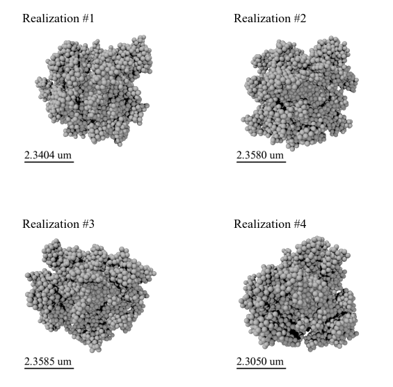
where partype is the particle type, size is the size of the aggregate (in units of the number of monomers), and amon is the monomer radius. The arguments that are used to call the function obey the same rules as the dust file name. By default, the command results in showing all realizations of each particle model. If you want to display only one of the realizations, add ireal in the argument (note: the realization index starts from 1, not 0):
[3]:
aggscatpy.view_particle(partype='CALP',size='4096',amon='100nm',ireal='1')
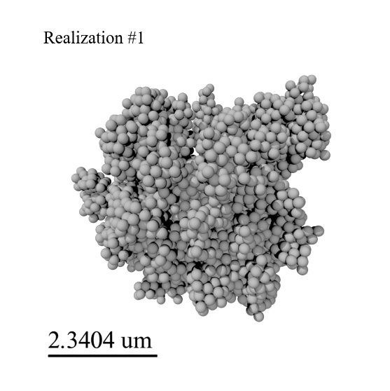
We can get a list of a possible combination between the amon and size arguments by using the get_sizelist function:
[4]:
aggscatpy.get_sizelist('CALP')
 Available amon and size for CALP
 amon='100nm' | size='8','16','32','64','128','256','512','1024','2048','4096'
 amon='200nm' | size='8','16','32','64','128','256','512'
 amon='400nm' | size='8','16','32','64'
The command to display irregular grains is
[5]:
aggscatpy.view_particle(partype='grs',size='1_6000')
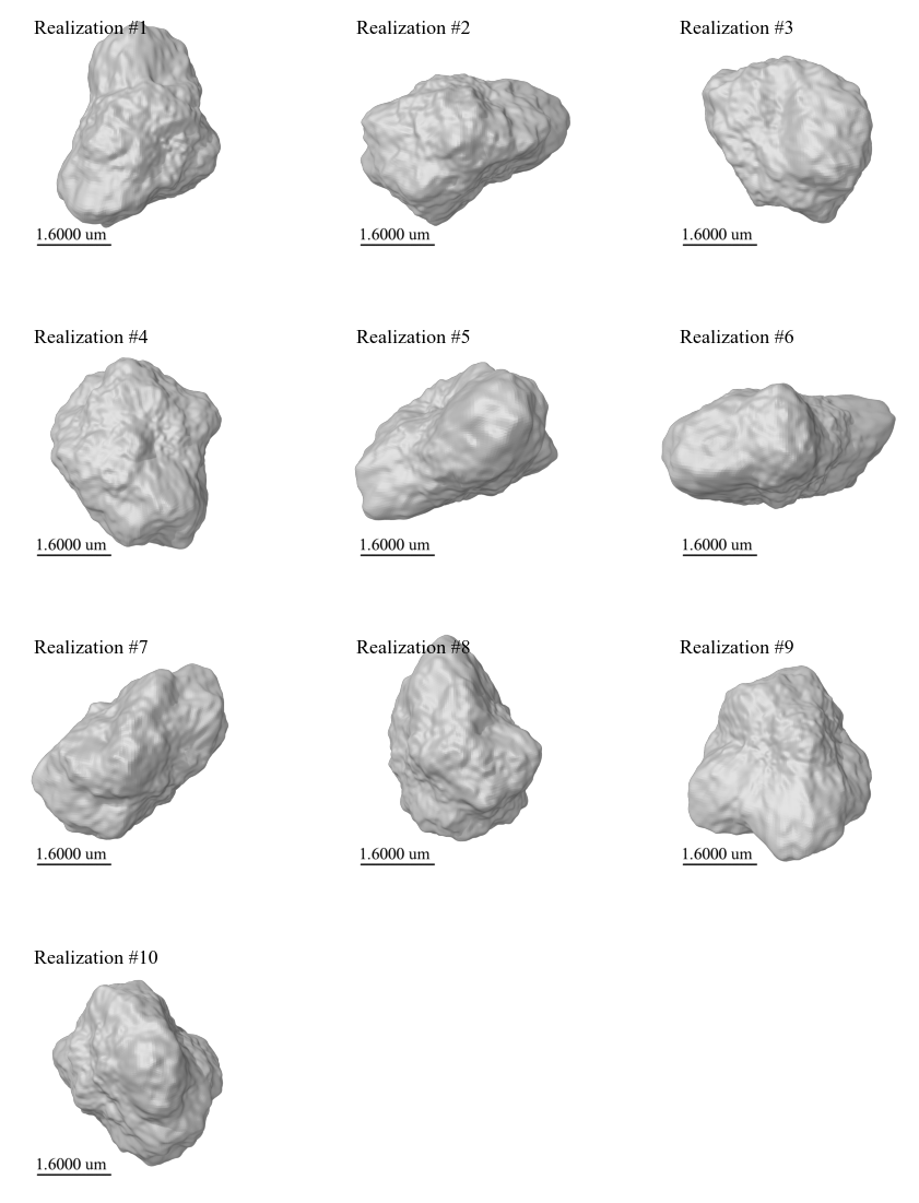
In this case, partype has to be 'grs'. The size argument represents the volume-equivalent radius of grains in units of microns (the decimal point needs to be replaced by the underscore). For example, size='1_6000' means that the volume-equivalent radius is \(1.6~\mu\)m. You can get a list of the available size arguments for irregular grains:
[6]:
aggscatpy.get_sizelist('grs')
[6]:
['0_2000',
 '0_2520',
 '0_3175',
 '0_4000',
 '0_5040',
 '0_6350',
 '0_8000',
 '1_0079',
 '1_2699',
 '1_6000']
Reading each dust model file
Basic formula
To read one of dustkapscatmat_XXX.inp stored in the AggScatVIR database, we can use the dustmodel class.
The basic command for reading an aggregate model is
[7]:
a=aggscatpy.dustmodel(partype='CALP',size='4096',amon='100nm',comp='amc')
where partype is the particle type, size is the size of the largest aggregate in the size distribution (in units of the number of monomers), amon is the monomer radius, and comp is the monomer composition. After running this command, the instance a will contain the physical and optical properties of the dust model of CALP_Nmax4096_100nm_amc.
The command for reading an irregular grain model is
[8]:
b=aggscatpy.dustmodel(partype='grs',size='1_6000',comp='org')
The size argument specifies the maximum volume-equivalent radius of grains.
By default, the dustmodel class reads a dust file with size distribution and no forward-scattering chopping. You can change these default settings by adding the dist and/or chop option(s) when calling the class. For example, if you want to switch off the size distribution, set dist=False (default: dist=True). If you want to have forward scattering chopping, set either chop='chop5' or chop='chop10' (default: chop='nochop'). chop5 and chop10 refer to
cases where the forward scattering peak is chopped at scattering angles below 5 or 10 degrees, respectively. The exemplary command for these cases are
[9]:
a2=aggscatpy.dustmodel(partype='CALP',size='4096',amon='100nm',comp='amc',dist=False,chop='chop5')
Check physical and optical properties
Each instance created by dustmodel contains the physical and optical properties of the dust model in its attributes (see Appendix C for the attributes).
We can display the physical properties of the dust particle stored in the instance a by using the dustspec function:
[10]:
aggscatpy.dustspec(a)
=============== Dust Parameters ================
 Model name = CALP_Nmax4096_100nm_amc
 Monomer radius           (um) = 0.10000
 Material density       (g/cc) = 1.7779
 -----Minimum aggregate in the distribution-----
 Number of monomers            = 8
 Volume-eq radius         (um) = 2.00000e-01
 Characteristic radius    (um) = 2.22916e-01
 Porosity                  (%) = 27.78
 -----Maximum aggregate in the distribution-----
 Number of monomers            = 4096
 Volume-eq radius         (um) = 1.60000e+00
 Characteristic radius    (um) = 2.34047e+00
 Porosity                  (%) = 68.05
 -----------------------------------------------
 Power-law index of size dist. = 3.50000e+00
 chop angle (deg)              = 0.00000e+00
================================================
Note that the above parameters are the averaged values for all realizations.
We can make some plots for the optical properties of the dust particle by using the showmodel function:
[11]:
aggscatpy.showmodel(a)
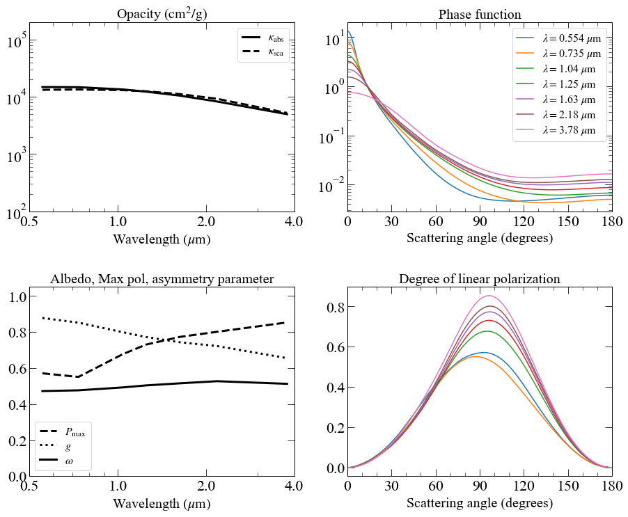
The above plots summarize the absorption and scattering opacities (\(\kappa_\mathrm{abs}\), \(\kappa_\mathrm{sca}\)) (left top), the single scattering albedo (\(\omega\)), the asymmetry parameter (\(g\)), and the maximum degree of linear polarization (\(P_\mathrm{max}\)) (left bottom), the scattering phase function (right top) and the degree of linear polarization (right bottom) at various wavelengths.
The showmodel function has some options that might be useful for you: (1) If you set opacity=False, the left top panel will be replaced by cross sections (\(\mu\mathrm{m}^2\)) instead of the opacity (\(\mathrm{cm}^2/\mathrm{g}\)) (2) If you set savefig=True, the plot will be saved. The file name will be generated automatically, but you can set your own file name by adding fn=your_favorate_filename.
If you would like to do a more flexible analysis, it is good to directly look into the values stored as attributes in each instance. For example, you can get the values of wavelength, opacity, and the asymmetry parameter:
[12]:
print('%13s '*4%("lambda","kabs","ksca","asym"))
for i in range(a.nlmd):
    print('%13.6e '*4%(a.lmd[i],a.kabs[i],a.ksca[i],a.asym[i]))
       lambda          kabs          ksca          asym
 5.540000e-01  1.478310e+04  1.324085e+04  8.782218e-01
 7.350000e-01  1.471897e+04  1.339719e+04  8.523817e-01
 1.040000e+00  1.345137e+04  1.305858e+04  7.994422e-01
 1.250000e+00  1.230322e+04  1.249605e+04  7.724140e-01
 1.630000e+00  1.047132e+04  1.113624e+04  7.433839e-01
 2.180000e+00  8.285653e+03  9.240539e+03  7.224008e-01
 3.780000e+00  4.970084e+03  5.227980e+03  6.553526e-01
The scattering angle grid is
[13]:
print(a.scatang)
[  0.   1.   2.   3.   4.   5.   6.   7.   8.   9.  10.  11.  12.  13.
  14.  15.  16.  17.  18.  19.  20.  21.  22.  23.  24.  25.  26.  27.
  28.  29.  30.  31.  32.  33.  34.  35.  36.  37.  38.  39.  40.  41.
  42.  43.  44.  45.  46.  47.  48.  49.  50.  51.  52.  53.  54.  55.
  56.  57.  58.  59.  60.  61.  62.  63.  64.  65.  66.  67.  68.  69.
  70.  71.  72.  73.  74.  75.  76.  77.  78.  79.  80.  81.  82.  83.
  84.  85.  86.  87.  88.  89.  90.  91.  92.  93.  94.  95.  96.  97.
  98.  99. 100. 101. 102. 103. 104. 105. 106. 107. 108. 109. 110. 111.
 112. 113. 114. 115. 116. 117. 118. 119. 120. 121. 122. 123. 124. 125.
 126. 127. 128. 129. 130. 131. 132. 133. 134. 135. 136. 137. 138. 139.
 140. 141. 142. 143. 144. 145. 146. 147. 148. 149. 150. 151. 152. 153.
 154. 155. 156. 157. 158. 159. 160. 161. 162. 163. 164. 165. 166. 167.
 168. 169. 170. 171. 172. 173. 174. 175. 176. 177. 178. 179. 180.]
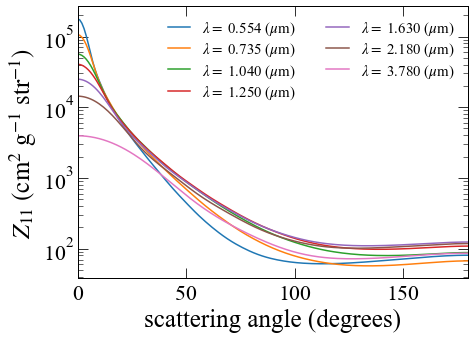
Each instance contains the scattering phase function (phase) and 6 scattering matrix elements (smat11,smat12,smat22,smat33,smat34,smat44) as its attributes. Note that the scattering matrix elements follow the RADMC-3D definition \(Z_{ij}\) (though you can change the definition into the Bohren & Huffman one if you want; see the next section for more information). Each of them is a function of wavelength and scattering angle, resulting in a two-dimensional
array. For example, \(Z_{11}(\lambda,\theta)\) has the shape of:
[14]:
print(a.smat11.shape)
(7, 181)
To fix the wavelength value, the first dimension should be fixed to the same index (note that the index 0 corresponds to the shortest wavelength):
[15]:
iwav=0
print('wavelength (um) =',a.lmd[iwav])
print(a.smat11[iwav,:])
wavelength (um) = 0.554
[1.78523701e+05 1.72076762e+05 1.54313366e+05 1.29350307e+05
 1.02329476e+05 7.77059918e+04 5.80906878e+04 4.40254779e+04
 3.45653906e+04 2.81956832e+04 2.35910583e+04 1.99552039e+04
 1.69623229e+04 1.45235619e+04 1.25808977e+04 1.10308479e+04
 9.74923875e+03 8.64216597e+03 7.66671589e+03 6.81441283e+03
 6.08339622e+03 5.46071838e+03 4.92454864e+03 4.45354507e+03
 4.03431975e+03 3.66028830e+03 3.32782113e+03 3.03245312e+03
 2.76826197e+03 2.52943988e+03 2.31199302e+03 2.11382100e+03
 1.93380792e+03 1.77096613e+03 1.62365691e+03 1.49021881e+03
 1.36866106e+03 1.25752151e+03 1.15558195e+03 1.06202720e+03
 9.76284542e+02 8.97925708e+02 8.26541315e+02 7.61695171e+02
 7.02873163e+02 6.49525719e+02 6.01067135e+02 5.56948310e+02
 5.16610929e+02 4.79575309e+02 4.45416373e+02 4.13847323e+02
 3.84689891e+02 3.57845984e+02 3.33254058e+02 3.10838706e+02
 2.90434396e+02 2.71863034e+02 2.54907267e+02 2.39364559e+02
 2.25080190e+02 2.11923313e+02 1.99800694e+02 1.88622796e+02
 1.78317009e+02 1.68818415e+02 1.60063005e+02 1.52006393e+02
 1.44602475e+02 1.37809215e+02 1.31578024e+02 1.25853434e+02
 1.20587034e+02 1.15729740e+02 1.11233669e+02 1.07058720e+02
 1.03176451e+02 9.95610613e+01 9.61988077e+01 9.30735846e+01
 9.01777024e+01 8.75010469e+01 8.50302105e+01 8.27590685e+01
 8.06742040e+01 7.87662024e+01 7.70201543e+01 7.54239170e+01
 7.39646475e+01 7.26281681e+01 7.14024737e+01 7.02765860e+01
 6.92443554e+01 6.82971010e+01 6.74282481e+01 6.66313619e+01
 6.59021268e+01 6.52355189e+01 6.46298134e+01 6.40794435e+01
 6.35835636e+01 6.31385302e+01 6.27427877e+01 6.23934658e+01
 6.20870720e+01 6.18220945e+01 6.15939791e+01 6.14023455e+01
 6.12440215e+01 6.11183206e+01 6.10230506e+01 6.09565973e+01
 6.09167990e+01 6.09043568e+01 6.09157808e+01 6.09507244e+01
 6.10087964e+01 6.10878845e+01 6.11884538e+01 6.13086688e+01
 6.14474816e+01 6.16053479e+01 6.17794697e+01 6.19726455e+01
 6.21806893e+01 6.24046256e+01 6.26430835e+01 6.28954983e+01
 6.31631301e+01 6.34425101e+01 6.37336046e+01 6.40379870e+01
 6.43531269e+01 6.46783742e+01 6.50129942e+01 6.53583050e+01
 6.57102859e+01 6.60714449e+01 6.64395286e+01 6.68148710e+01
 6.71966115e+01 6.75839667e+01 6.79774189e+01 6.83752527e+01
 6.87785084e+01 6.91855566e+01 6.95966571e+01 7.00101217e+01
 7.04262912e+01 7.08453499e+01 7.12653040e+01 7.16872892e+01
 7.21094206e+01 7.25318912e+01 7.29531296e+01 7.33732958e+01
 7.37924770e+01 7.42078859e+01 7.46220828e+01 7.50311903e+01
 7.54364010e+01 7.58354784e+01 7.62278272e+01 7.66127093e+01
 7.69869196e+01 7.73530694e+01 7.77063968e+01 7.80482375e+01
 7.83746383e+01 7.86850360e+01 7.89770127e+01 7.92512559e+01
 7.95023617e+01 7.97313405e+01 7.99342576e+01 8.01104834e+01
 8.02576310e+01 8.03740646e+01 8.04586167e+01 8.05095686e+01
 8.05255704e+01]
Thus \(Z_{11}(\lambda,\theta)\) for this dust model looks like this:
[16]:
import matplotlib
import matplotlib.pyplot as plt

fig, ax =plt.subplots(figsize=(7,5))
ax.set_ylabel('$Z_{11}~(\mathrm{cm}^2~\mathrm{g}^{-1}~\mathrm{str}^{-1})$')
ax.set_xlim(0,180)
ax.set_yscale('log')
ax.set_xlabel('scattering angle (degrees)')
for iwav in range(a.nlmd):
    label='$\lambda=$ %5.3f ($\mu\mathrm{m}$)'%a.lmd[iwav]
    ax.plot(a.scatang,a.smat11[iwav,:],label=label)
ax.legend(fontsize=15,ncol=2,frameon=False)
[16]:
<matplotlib.legend.Legend at 0x7f7fe530c190>
Scattering matrix in Bohren & Huffman’s definition
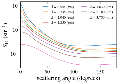
It is sometimes useful to have the scattering matrix elements in the Bohren & Huffman definition. You can switch the definition into Bohren & Huffman’s one by setting smatBH=True when calling the dustmodel class:
[17]:
abh=aggscatpy.dustmodel(partype='CALP',size='4096',amon='100nm',comp='amc',smatBH=True)
All the values in the attributes (smat11,smat12,smat22,smat33,smat34,smat44) have been replaced by the ones in Bohren & Huffman’s definition (so smat11 now contains \(S_{11}\) instead of \(Z_{11}\)). Thus \(S_{11}(\lambda,\theta)\) looks like this:
[18]:
fig, ax =plt.subplots(figsize=(7,5))
ax.set_ylabel('$S_{11}~(\mathrm{str}^{-1})$')
ax.set_xlim(0,180)
ax.set_yscale('log')
ax.set_xlabel('scattering angle (degrees)')
for iwav in range(abh.nlmd):
    label='$\lambda=$ %5.3f ($\mu\mathrm{m}$)'%abh.lmd[iwav]
    ax.plot(abh.scatang,abh.smat11[iwav,:],label=label)
ax.legend(fontsize=15,ncol=2,frameon=False)
[18]:
<matplotlib.legend.Legend at 0x7f7fc0ce5f70>
Perform size distribution averaging and apply forward scattering chopping
This database contains the optical properties averaged over a particle-size distribution. The size distribution is assumed to have a simple power-law form:
where \(a_\mathrm{V}\) is the volume-equivalent radius and \(n(a_\mathrm{V})da_\mathrm{V}\) is the number density of particles within a radius range of \([a_\mathrm{V},a_\mathrm{V}+da_\mathrm{V}]\). For aggregates,
where \(N_\mathrm{min}\) and \(N_\mathrm{max}\) are the number of monomers of the smallest and largest aggregate in the size distribution, respectively. By default, we assume \(q=3.5\), \(N_\mathrm{min}=8\) for aggregates, and \(a_\mathrm{V,min}=0.2~\mu\)m for irregular grains.
However, you may be interested in the optical properties for different size distributions, such as \(q\ne3.5\) . By using distaverage, we can perform size distribution averaging of the optical properties with user-specified values of \(a_\mathrm{min}\), \(a_\mathrm{max}\), and \(q\). In addition, it can also be used to apply forward scattering chopping with a user-specified chop angle.
Basic formula
The basic command is
[19]:
d=aggscatpy.distaverage(partype='CALP',sizemin='8',sizemax='4096',comp='amc',amon='100nm',powind=3.5)
The newly created instance d contains the distribution-averaged optical properties. The sizemin and sizemax represent the smallest and largest aggregates in the distribution in units of the number of monomers, respectively, and powind is the power-law index \(q\).
The command for irregular grains is
[20]:
e=aggscatpy.distaverage(partype='grs',sizemin='0_2000',sizemax='1_6000',comp='org', powind=3.5)
As with the case of dustmodel, an instance created by distaverage can be substituted into functions: dustspec(), showmodel(), and write_data() (the last function will be introduced later).
Since the parameters used above are exactly the same as the default size distribution, the results have to agree with those contained in the default dust files. As shown below, these two are in perfect agreement.
[21]:
for i in range(a.nlmd):
    print('wavelength = %6.3f'%(a.lmd[i]))
    print('     %-11s = %13.6e %13.6e %13.6e %13.6e'\
          %("tabulated",a.kabs[i],a.ksca[i],a.asym[i],a.pmax[i]))
    print('     %-11s = %13.6e %13.6e %13.6e %13.6e'\
          %("recomputed",d.kabs[i],d.ksca[i],d.asym[i],d.pmax[i]))
wavelength =  0.554
     tabulated   =  1.478310e+04  1.324085e+04  8.782218e-01  5.710268e-01
     recomputed  =  1.478310e+04  1.324085e+04  8.782218e-01  5.710268e-01
wavelength =  0.735
     tabulated   =  1.471897e+04  1.339719e+04  8.523817e-01  5.509632e-01
     recomputed  =  1.471897e+04  1.339719e+04  8.523817e-01  5.509632e-01
wavelength =  1.040
     tabulated   =  1.345137e+04  1.305858e+04  7.994422e-01  6.768769e-01
     recomputed  =  1.345137e+04  1.305858e+04  7.994422e-01  6.768769e-01
wavelength =  1.250
     tabulated   =  1.230322e+04  1.249605e+04  7.724140e-01  7.304774e-01
     recomputed  =  1.230322e+04  1.249605e+04  7.724140e-01  7.304774e-01
wavelength =  1.630
     tabulated   =  1.047132e+04  1.113624e+04  7.433839e-01  7.730357e-01
     recomputed  =  1.047132e+04  1.113624e+04  7.433839e-01  7.730357e-01
wavelength =  2.180
     tabulated   =  8.285653e+03  9.240539e+03  7.224008e-01  8.013906e-01
     recomputed  =  8.285653e+03  9.240539e+03  7.224008e-01  8.013906e-01
wavelength =  3.780
     tabulated   =  4.970084e+03  5.227980e+03  6.553526e-01  8.534474e-01
     recomputed  =  4.970084e+03  5.227980e+03  6.553526e-01  8.534474e-01
Examples
If you want the size distribution between \(N_\mathrm{min}=128\) to \(N_\mathrm{max}=2048\) with the default power-law index (\(q=3.5\)):
[22]:
d=aggscatpy.distaverage(partype='CALP',sizemin='128',sizemax='2048',comp='amc',amon='100nm')
… and change the power-law index to \(q=2.5\):
[23]:
d=aggscatpy.distaverage(partype='CALP',sizemin='128',sizemax='2048',\
              comp='amc',amon='100nm',powind=2.5)
… and change the chop angle to 7 degrees:
[24]:
d=aggscatpy.distaverage(partype='CALP',sizemin='128',sizemax='2048',\
              comp='amc',amon='100nm',powind=2.5,chopang=7)
If you set \(N_\mathrm{min}=N_\mathrm{max}\), the results will be the same as the single-sized case.
You can also change the definition of the scattering matrix:
[25]:
dbh=aggscatpy.distaverage(partype='CALP',sizemin='128',sizemax='2048',comp='amc',amon='100nm', smatBH=True)
Writing files
Once you have generated the optical properties with a new particle-size distribution and/or chop angle, you may wish to save them as a RADMC-3D readable format. To do this, you can use the write_data function. An instance created by either the dustmodel or distaverage class can be passed to the write_data function to write a new file.
Suppose you have already created an instance d, then you can type:
[26]:
aggscatpy.write_data(d)
writing ... dustkapscatmat_CALP_Nmin128_Nmax2048_pow2.5_100nm_amc_chop7.0.inp
The filename will be automatically generated based on the minimum and maximum particle sizes, power-law index, and chopping angle (if non-zero). You can also modify the filename by setting the fn option if you want.
Without any options, the generated file will have a standard ‘dustkapscatmat_XXX’ format.
Important
The definition of the scattering matrix to be written in the file will be the same as the one defined in each instance. Since the above instance d has the scattering matrix with the RADMC definition, the generated file contains \(Z_{ij}\). In this case, the generated file is directly readable by RADMC-3D.
Conversely, if you have created an instance that has the scattering matrix in Bohren & Huffman’s definition, the following will happen:
[27]:
aggscatpy.write_data(dbh)
writing ... dustkapscatmat_CALP_Nmin128_Nmax2048_pow3.5_100nm_amc.out
In this case, the structure of the generated file is the same, but the file contains \(S_{ij}\) instead of \(Z_{ij}\). To avoid confusion, the file extension has been changed from .inp to .out so that the file is not readable by RADMC-3D anymore. You can also check the definition in the header part of each generated file.
If you are only interested in the angle-integrated quantities (opacity, asymmetry parameter, …), you can add output='dustkappa':
[28]:
aggscatpy.write_data(a,output='dustkappa')
writing ... dustkappa_CALP_Nmax4096_100nm_amc.out
The generated file now only contains the angle-integrated quantities and not scattering matrix elements. If you are interested in cross sections instead of opacity, you can add the following option so that the output file will contain cross sections (\(\mu\mathrm{m}^2\)):
[29]:
aggscatpy.write_data(a,output='dustkappa', opacity=False)
writing ... dustkappa_CALP_Nmax4096_100nm_amc.out
Conversely, if you are only interested in scattering matrix elements, add output='smat':
[30]:
aggscatpy.write_data(a,output='smat')
writing ... scatmat_CALP_Nmax4096_100nm_amc_lmd0.554um.out
writing ... scatmat_CALP_Nmax4096_100nm_amc_lmd0.735um.out
writing ... scatmat_CALP_Nmax4096_100nm_amc_lmd1.04um.out
writing ... scatmat_CALP_Nmax4096_100nm_amc_lmd1.25um.out
writing ... scatmat_CALP_Nmax4096_100nm_amc_lmd1.63um.out
writing ... scatmat_CALP_Nmax4096_100nm_amc_lmd2.18um.out
writing ... scatmat_CALP_Nmax4096_100nm_amc_lmd3.78um.out
This command will generate some files; the number of files to be generated will be the same as the number of the wavelength grid (at most 7). If you do not need all wavelengths, you can limit the wavelength you want by adding an option:
[31]:
aggscatpy.write_data(a,output='smat',wlist=[1.25,1.63])
writing ... scatmat_CALP_Nmax4096_100nm_amc_lmd1.25um.out
writing ... scatmat_CALP_Nmax4096_100nm_amc_lmd1.63um.out
Reloading a dustkapscatmat_XXX file generated by this tool
The dustmodel class can read a file given in the format either dustkapscatmat_XXX.inp or dustkapscatmat_XXX.out generated by aggscatpy. To do so, you just need to specify the relative path to the file when calling:
[32]:
d2=aggscatpy.dustmodel(filename='./dustkapscatmat_CALP_Nmin8_Nmax2048_pow3.5_100nm_amc.out')
...reading ./dustkapscatmat_CALP_Nmin8_Nmax2048_pow3.5_100nm_amc.out
Example analysis
Comparing phase functions of different fractal dimensions
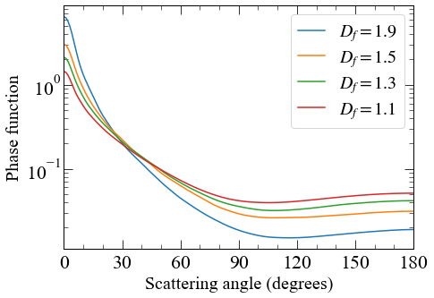
For example, let’s investigate how the total-intensity phase function of aggregates changes with fractal dimension at the \(H\) band wavelength (\(\lambda=1.63~\mu\)m).
To do so, first create some lists:
[33]:
pt=['FA19','FA15', 'FA13','FA11'] # a list of particle types
nmono=['2048','512', '256','128']      # a list of the number of monomers
label=['$D_f=1.9$','$D_f=1.5$','$D_f=1.3$','$D_f=1.1$'] # a list of labels for lenged
where we have assumed that a smaller number of monomers for a lower fractal dimension to approximately fix the aggregate radius. To check the characteristic radius of an aggregate, you can use the get_radius_and_porosity function
[34]:
for i in range(len(pt)):
    ac,por=aggscatpy.get_radius_and_porosity(pt[i],'100nm',nmono[i])
    print('Particle Type: %4s'%pt[i],' Number of monomers = %4s'%nmono[i],' agg radius = %5.2f um'%ac)
Particle Type: FA19  Number of monomers = 2048  agg radius =  6.72 um
Particle Type: FA15  Number of monomers =  512  agg radius =  6.60 um
Particle Type: FA13  Number of monomers =  256  agg radius =  6.73 um
Particle Type: FA11  Number of monomers =  128  agg radius =  6.56 um
Now we confirmed that the four aggregates have approximately the same characteristic radius: \(a_\mathrm{c}=6.645\pm0.085~\mu\)m. Then, let’s plot the phase function for those models.
[35]:
iwav=4 # to fix wavelength at lambda=1.630 um

fig, ax =plt.subplots(figsize=(7,5))
ax.set_ylabel('Phase function',fontsize=20)
aggscatpy.plots.set_ang_vs_phase(ax)
for i in range(len(pt)):
    a=aggscatpy.dustmodel(partype=pt[i],size=nmono[i],amon='100nm',comp='amc')
    print('Reading dust model ... ',a.model)
    print('---> wavelength=%5.2f (um)'%a.lmd[iwav], 'maximum aggregate radius = %5.2f (um)'%a.acmax)
    ax.plot(a.scatang,a.phase[iwav,:],label=label[i])
ax.legend(fontsize=20,loc='best')
Reading dust model ...  FA19_Nmax2048_100nm_amc
---> wavelength= 1.63 (um) maximum aggregate radius =  6.72 (um)
Reading dust model ...  FA15_Nmax512_100nm_amc
---> wavelength= 1.63 (um) maximum aggregate radius =  6.60 (um)
Reading dust model ...  FA13_Nmax256_100nm_amc
---> wavelength= 1.63 (um) maximum aggregate radius =  6.73 (um)
Reading dust model ...  FA11_Nmax128_100nm_amc
---> wavelength= 1.63 (um) maximum aggregate radius =  6.56 (um)
[35]:
<matplotlib.legend.Legend at 0x7f7fc0f54d00>
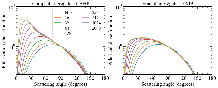
Polarization phase functions
Let’s give you one more example. In this example, we will see how the polarization phase function depends on aggregate radius and structure. Similar to the above example, we first make some lists:
[36]:
nmono=['8','16','32','64','128','256','512','1024','2048'] # a list of the number of monomers
label=['N=8','16','32','64','128','256','512','1024','2048'] # a list of labels for lenged
Then, read and plot the dust models iteratively in the loop:
[37]:
iwav=4 # to fix wavelength at 1.630 um
iangn=90 # a scattering angle used for normalization

fig, (ax1,ax2) =plt.subplots(1,2,figsize=(14,5))
aggscatpy.plots.set_ang_vs_phase(ax1)
aggscatpy.plots.set_ang_vs_phase(ax2)
ax1.set_ylabel('Polarization phase function',fontsize=20)
ax1.set_ylim(2.0e-1,10)
ax1.set_title('Compact aggregates: CAHP',fontsize=20)
ax2.set_ylabel('Polarized phase function',fontsize=20)
ax2.set_ylim(2.0e-1,10)
ax2.set_title('Fractal aggregates: FA19',fontsize=20)
for i in range(len(nmono)):
    a1=aggscatpy.dustmodel(partype='CAHP',size=nmono[i],amon='100nm',comp='org')
    a2=aggscatpy.dustmodel(partype='FA19',size=nmono[i],amon='100nm',comp='org')
    ax1.plot(a1.scatang,a1.smat12[iwav,:]/a1.smat12[iwav,iangn],label=label[i])
    ax2.plot(a2.scatang,a2.smat12[iwav,:]/a2.smat12[iwav,iangn],label=label[i])
ax1.legend(fontsize=18,ncol=2,loc='best')
[37]:
<matplotlib.legend.Legend at 0x7f7fe52dcca0>